Optimizing SRNN

14.06.2020

1. Introduction

In this writeup, I will explain how I optimized the running time of a neural network called SRNN(Shuffling Recurrent Neural Network).

This work was originally developed several years ago as part of an academic project, I hope that someone will find this work helpful, please reach out for any questions/comments.

We begin with background on the neural network itself, and then move to optimization iterations of profiling followed by code modifications. Each iteration results in a faster version while preserving functionality.

Each iteration involves the following:

1. Profiling - analyzing the running the time of every component, identifying bottle-necks and places to intervene.
2. Implementation - writing and modifying CUDA kernels and PyTorch code.

This article focuses on the forward function. Backward-pass optimization was also done and might be covered separately in a future post.

By combining operator fusion, and memory-access optimization, the optimized SRNN forward achieved up to 5x faster execution while maintaining identical output.

The following figure shows the runtime improvement on a common GPU used for training and inference.

Figure 1. Runtime vs batch size and sequence length.
Original implementation of SRNN (orange) is slower than the baseline network GRU (Gated Recurrent Unit, blue) which is slower than the optimized version of SRNN (green).

1.1. Key Takeaways

• When performance is memory-bound, combining multiple element-wise operations into a single CUDA kernel achieves great improvements.
• Profiling is valuable both for guiding where to optimize and benchmark our effort. This saves time.
• Eliminating Python-level slicing and stacking can yield major improvements.

1.2. Possible Improvements

• Profile with Nsight Systems / Nsight Compute to verify that memory access patterns remain efficient (coalesced reads, balanced occupancy), even though the work intentionally avoids device-specific tuning.

2. Background

The Shuffling Recurrent Neural Network (SRNN) is a recurrent architecture introduced by Rotman and Wolf to address instabilities in training deep RNNs, such as exploding and vanishing gradients.
It modifies the standard Recurrent Neural Network (RNN) recurrence by applying a circular shift to the hidden state before combining it with the current input.
This simple change encourages better gradient flow and spatial information mixing between hidden units.

SRNN’s PyTorch implementation introduces significant overhead.
Each time step performs multiple element-wise operations (roll, add, relu) and Python-level tensor manipulations (stack, select), which quickly dominate runtime as sequence length increases.

2.1. Forward Function Overview

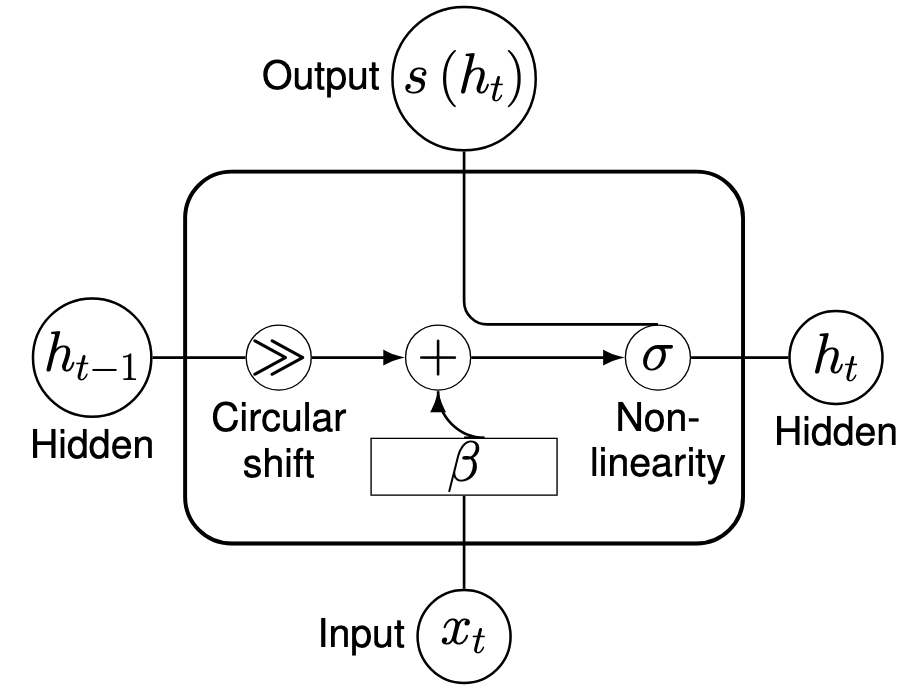
Figure 2. Overview of SRNN forward computation.

Step by Step Explanation

Short explanation of the forward function, given an input xt and hidden state ht-1:

1. Apply subnetwork b on xt
2. Apply circular shift on ht-1
3. For ht-1={a1, a2, a3, ..., an}the results would be {an , a1, a2, a3, ..., an-1}
4. Add the results of steps 1 and 2 element-wise.
5. Apply Non-linearity(i.e. relu) to the result of step 3

The forward step of the SRNN can be expressed as:

\[ h_t = \text{ReLU}\left( \beta(x_t) + \text{circ_shift}(h_{t-1}) \right) \]

where \( h_t \) is the hidden state at time \( t \), \( x_t \) is the input at time \( t \), \(\beta\) is a subnetwork that processes the input, and \(\text{circ_shift}(\cdot)\) denotes a circular shift operation on the hidden state vector.

The subnetwork β(xₜ) is a simple fully connected followed by a gate as seen in the image below.

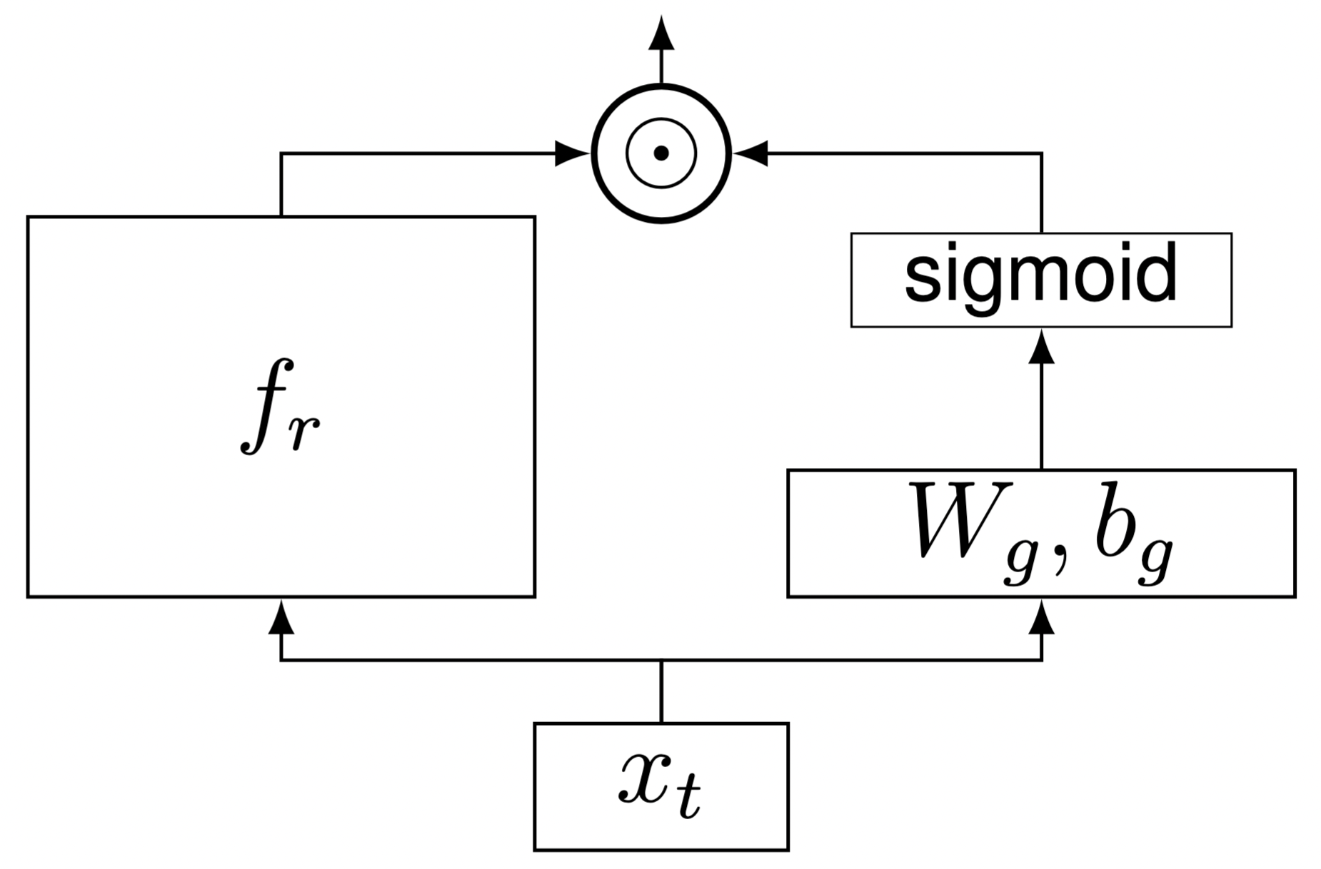
Figure 3. Overview of the subnetwork forward computation.

Below is a baseline PyTorch implementation SRNN forward function, the steps in the comments refer to the details section below Figure 3:

def forward(self, x: torch.Tensor, hidden: Optional[torch.Tensor] = None):
   batch_size, seq_len, inp_size = x.shape

   # Subnetwork b.
   b = self.fc(x) # Step 1
   sig_alphas = torch.sigmoid(self.fc2(x)) # Steps 2 + 3
   b = b * sig_alphas

   # Calculate hidden state of first input in sequence. Step 4
   if hidden is not None:
       outputs = [torch.relu(b[:, 0] + torch.roll(hidden, 1, -1))]
   else:
       outputs = [torch.relu(b[:, 0])]

   # Calculate hidden state of the rest of the inputs. Step 4
   for i in range(1, seq_len):
       outputs.append(torch.relu(b[:, i] + torch.roll(outputs[-1], 1, -1)))

   outputs = torch.stack(outputs, 1)
   hidden = outputs[:, -1, :]

   outputs = outputs.squeeze(2)

Step by Step Explanation

The forward implementation accepts a 3-dimensional input - (batch_size, sequence_length, input_size) and a 2-dimensional hidden state - (batch_size, hidden_size).

• Step 1 of the forward function is applied to all the inputs of all the sequences of all the batches in parallel since it’s not dependent on any previous calculations. In terms of optimization it is probably as fast as it can be.
• The for loop applies steps 2 - 4 for all the sequence, calculating the hidden states one after the other until the final hidden state is calculated and returned as the output.
• Each line in the implementation works across all the batches, this enables pytorch to parallelize its calculations. So if we had batch_size = 32, and sequence length = 200, the for loop would run 200 times, in each time, it would roll 32 hidden states and add them to 32 results from step 1.

3. Methodology

I've used Pytorch + CUDA in this work and PyTorch's built-in torch.autograd.profiler for profiling.

The profiling setup used the following dimensions: - Batch size: 1 - Input size: 128 - Hidden size: 512 - Output size: 64 - Sequence length: 2000

I've also tested other batch sizes and dimensions but didn't include them for simplicity.

The most important part - Test were written to make sure that outputs remain bit-exact as they were before any modifications for both forward and backward optimization.

All benchmarks were run on an NVIDIA MX150 GPU with CUDA 10.2 and PyTorch 1.4.0”

4. Iteration #1

4.1. Profiling

Profiling results:

Name	CUDA total %	CUDA total	CUDA time avg	Number of Calls	Input size
add	28.05%	2.074s	10.377us	199900	[[1 512] [1 512]]
relu	26.64%	1.970s	9.856us	199900	[[1 512]]
roll	24.02%	1.776s	8.881us	200000	[[1 512]]
select	12.55%	928.231ms	4.639us	200100	[[1 2000 512]]
stack	4.28%	316.819ms	3.168ms	100	[]
matmul	0.46%	34.170ms	341.696us	100	[[1 2000 128] [128 512]]
* more insignificant rows removed

Run time mean over 100 runs:

Version	Run time(s)
v0	0.107

Takeaways:

1. add(), roll() and relu() take ~75% of the total running time when batch size is 1
2. select() and stack() take ~16% of the total running time when batch size is 1

We are going to write a cuda kernel and here are possible optimizations:

1. Fuse roll-sum-relu operators - those three always come one after the other and all of them are element wise operators, which makes them a great candidate for fusion. Using a single memory access, we can do all of them together. Since we have to pay for at least one memory access, which we assume is the most expensive action
2. Eliminate the roll() - Instead of doing \(f\left(x_t\right)=x_t+\text{roll}\left(h_t - 1\right) \) and actually rolling \(h_t - 1\) and by that, moving memory, we can do \(f\left(x_t\right)\left[i\right] = x_t\left[i\right] + h_t\left[i + 1\right]\). Which is much more efficient.
3. Eliminate select and stack by referencing memory directly using indexing - instead of taking a chunk of memory and “looking” at it differently by changing the strides(which select() does), we can just access the memory directly.

4.2. Implementation v1

We start by addressing points 1 and 2. I wrote a cuda function and compiled it as a torchscript extension(now deprecated).

The function is called roll_sum_relu() and does the following:

1. Using a single memory access, it does the three operations as discussed in the previous section.
2. Using random access with h_idx, we avoid the roll() operator.

template <typename scalar_t>
__global__ void roll_sum_relu_cuda_kernel(
    const torch::PackedTensorAccessor<scalar_t,2,torch::RestrictPtrTraits,size_t> input,
    const torch::PackedTensorAccessor<scalar_t,2,torch::RestrictPtrTraits,size_t> hidden,
    torch::PackedTensorAccessor<scalar_t,2,torch::RestrictPtrTraits,size_t> res) {

    // batch index
    const int n = blockIdx.y;     
    // column index
    const int c = blockIdx.x * blockDim.x + threadIdx.x;
    if (c < input.size(1)) {
        const int h_idx = (c == 0) ? input.size(1) - 1 : c - 1;
        res[n][c] = relu(input[n][c] + hidden[n][h_idx]);
  }
}

The modified python code that now uses the compiled cuda function:

def forward(self, x, hidden: Optional[torch.Tensor] = None):
    batch_size, seq_len, inp_size = x.shape

    b = self.fc(x)
    sig_alphas = torch.sigmoid(self.fc2(x))
    b = b * sig_alphas

    if hidden is not None:
        outputs = [torch.ops.my_cuda_ops.roll_sum_relu(b[:, 0], hidden)]
    else:
        outputs = [torch.relu(b[:, 0])]

    for i in range(1, seq_len):
        outputs.append(torch.ops.my_cuda_ops.roll_sum_relu(b[:, i], outputs[-1]))

    outputs = torch.stack(outputs, 1)
    hidden = outputs[:, -1, :]

    outputs = outputs.squeeze(2)

    return outputs, hidden

5. Iteration #2

Now we'll work on point 3 from the previous section - slice, select and stack

5.1. Profiling

Name	CUDA total %	CUDA total	CUDA time avg	Number of Calls
roll_sum_relu	55.31%	2.778s	13.945us	199200
slice	16.95%	851.481ms	4.255us	200100
select	16.66%	836.835ms	4.182us	200100
stack	5.79%	291.024ms	2.910ms	100
* more insignificant rows removed

Run time mean over 100 runs:

Version	Run time(s)
v0	0.107
v1	0.046

Takeaways:

1. The roll_sum_relu operator is now responsible for 55% percent of the running time.
2. Slice+select+stack are now responsible for ~40% of the running time.

5.2. Implementation v2

The line that interests us is:

outputs.append(torch.ops.my_cuda_ops.roll_sum_relu(b[:, i], outputs[-1]))

For each sequence \(i\) we slice from \(b\) all the batches. For example, let b be a 3-dimenstional tensor of shape (32, 20, 64) - (batch size, sequence length, hidden state size). The expression \(b[:, 0]\) will give a shape (32, 64) which is the hidden states of all the batches after the first input in the sequence. If we have access to b we don’t really need to slice, we can just access the elements using their indices.

To solve this, I’ve inserted the loop into the cuda code and accessed the tensors using indices instead of slicing them.

Here’s how the forward function looks after using the upgraded roll_sum_relu() function:

def forward(self, x, hidden: torch.Tensor):
    b = self.fc(x)
    sig_alphas = torch.sigmoid(self.fc2(x))
    b = b * sig_alphas

    outputs = torch.ops.my_cuda_ops.roll_sum_relu(b, hidden)
    hidden = outputs[:, -1, :]

    return outputs, hidden

6. Final Profiling

Name	CUDA total %	CUDA total	CUDA time avg	Number of Calls	Input Shapes
roll_sum_relu	88.11%	1.906s	19.055ms	100	[[1 2000 512] [1 512]]
add_	1.87%	40.365ms	201.826us	200	[[1 2000 512] [512] []]
matmul	1.60%	34.660ms	346.604us	100	[[1 2000 128] [128 512]]
mm	1.51%	32.665ms	326.655us	100	[[2000 128] [128 512]]
FusionGroup	1.40%	30.246ms	302.460us	100	[]
matmul	1.05%	22.764ms	227.637us	100	[[1 2000 64] [64 512]]
* more insignificant rows removed

Run time mean over 100 runs:

Version	Run time(s)
v0	0.107
v1	0.046
v2	0.021

We’ve eliminated all the slice/select/stack operators and achieved 5x speedup overall.